Cooling during CO2 Injection into a Gas Reservoir

Context

When a real gas expands from a high to a low pressure at constant enthalpy, its temperature changes. This is the Joule-Thomson (JT) effect. For CO2 at reservoir conditions the gas cools when it expands. During carbon sequestration, CO2 is injected into a depleted natural gas reservoir and the pressure drops steeply between the wellbore and the reservoir, so JT cooling may occur close to the injection well. If it were large, it could lead to CO2 or CH4 hydrate formation, to freezing of the residual water (with a loss of injectivity), or to thermal stresses able to fracture the formation.

(Oldenburg, 2007) used the TOUGH2/EOS7C simulator to quantify the magnitude of this cooling. The model was first verified against the classical JT expansion experiment, and was then applied to an idealized one-dimensional radial gas reservoir with constant-rate CO2 injection. The study showed that the cooling grows when the permeability decreases (a larger pressure drop is required to inject the same mass of CO2), and that it is partly compensated by the heat released by the rock matrix and the residual water.

This example reproduces the lowest-permeability case of the paper, $k = 5\times 10^{-15}$ m² (5 mD), whose results are shown in the paper. It is the case with the strongest cooling among the constant-rate injections with an injection temperature equal to the reservoir temperature, and therefore the most demanding one for the thermal formulation. It can serve as a validation of the thermal compositional multiphase flow solver of GEOS, in particular of the coupling between

a real-gas equation of state, which provides the enthalpy of the CO2-CH4-H2O mixture and thus the JT coefficient,
the energy balance, including the advection of enthalpy, the heat stored in the rock and in the immobile water, and conduction,
thermal wells with prescribed mass and volumetric rates.

Brief case description

Reservoir model of the paper

The paper considers an idealized depleted gas reservoir, with the geometry and the properties given in the paper. It is represented by a one-dimensional radially symmetric system, 50 m thick and 1130 m in radius, as illustrated below.

injection well (r = 0)  --->  CO2-rich gas  | CH4-rich gas  --->  production (r ~ 1100 m)

The reservoir is initially filled with methane at 50 bar and 45 °C. The water is immobile (the water saturation is equal to the residual saturation $S_{lr} = 0.2$ ), and the only mobile phase is the gas. Pure CO2 is injected at a constant rate of 3 kg/s and at the reservoir temperature. Methane is produced at the outer boundary, at 0.56 kg/s. The system is closed: no fluid or heat crosses the outer boundary. Because the injection temperature is equal to the initial reservoir temperature, every temperature change in the reservoir is caused by the JT effect (attenuated by the heat provided by the rock and the water), which makes this setup well suited to isolate and validate this effect.

The parameters of the problem are summarized in the following table.

Table 1 Parameters of the problem
Parameter	Value
Geometry	1D radial, $R = 1130$ m, thickness 50 m GEOS is modeled as a 1° sector, $r \in [0.1, 1130]$ m.
Permeability	$5\times 10^{-15}$ m² (5 mD)
Porosity	0.30
Rock volumetric heat capacity	$2.6\times 10^{6}$ J/m³/K
Thermal conductivity	2.51 W/m/K
Residual saturations	$S_{lr} = 0.2$ (water), $S_{gr} = 0.01$ (gas)
Relative permeability	Corey curves
Initial pressure	50 bar ( $5\times 10^{6}$ Pa)
Initial temperature	45 °C (318.15 K)
Initial fluids	CH4 gas, water at $S_l = S_{lr} = 0.2$ GEOS initializes this via mass fractions: $z_{CO_2} = 0$ , $z_{CH_4} = 0.115401$ , $z_{H_2O} = 0.884599$ .
CO2 injection	3 kg/s of CO2 at 45 °C
CH4 production	0.56 kg/s at the outer boundary (1100 m)
Simulated time	15 years
Equation of state	Peng-Robinson for the gas phase The paper uses EOS7C/GasEOS, while GEOS explicitly uses Søreide-Whitson for the aqueous phase.

Input base

This benchmark test is based on the XML file located below:

inputFiles/compositionalMultiphaseFlow/benchmarks/jouleThomsonCooling/jouleThomsonCooling.xml

The mesh is a thin wedge of cylinder (InternalWellbore), 1° wide (theta from -0.5° to 0.5°). The 109 radial cells are defined explicitly through the radius and nr arrays: the cell size grows geometrically with the distance to the injection well (the ratio between successive radii decreases from 1.2 close to the well to about 1.08 at the outer boundary), which refines the mesh where the pressure and temperature gradients are the strongest. The 360° of the paper are accounted for by dividing all the well rates by 360.

  <Mesh>
    <InternalWellbore
      name="mesh"
      elementTypes="{ C3D8 }"
      radius="{
        0.1, 0.12, 0.141606, 0.164948, 0.190164, 0.217405, 0.246834, 0.278627, 0.312973, 0.350077, 0.390162, 0.433465,
        0.480247, 0.530785, 0.585383, 0.644365, 0.708085, 0.776922, 0.851287, 0.931625, 1.01841, 1.11217, 1.21347,
        1.32289, 1.4411, 1.56881, 1.70678, 1.85582, 2.01683, 2.19078, 2.3787, 2.5817, 2.80102, 3.03794, 3.2939,
        3.57041, 3.86912, 4.19183, 4.54046, 4.91708, 5.32396, 5.7635, 6.23836, 6.75134, 7.30553, 7.90422, 8.551,
        9.24972, 10.0046, 10.82, 11.701, 12.6527, 13.6808, 14.7915, 15.9914, 17.2877, 18.6881, 20.201, 21.8353, 23.601,
        25.5084, 27.569, 29.7951, 32.2, 34.798, 37.6047, 40.6368, 43.9124, 47.4511, 51.274, 55.404, 59.8656, 64.6855,
        69.8925, 75.5177, 81.5947, 88.1598, 95.2521, 102.914, 111.191, 120.133, 129.793, 140.23, 151.504, 163.683,
        176.841, 191.056, 206.412, 223.001, 240.923, 260.284, 281.2, 303.796, 328.207, 354.578, 383.067, 413.844,
        447.093, 483.012, 521.816, 563.736, 609.023, 657.948, 710.801, 767.899, 829.583, 896.221, 968.211, 1045.98,
        1130
      }"
      nr="{
        1, 1, 1, 1, 1, 1, 1, 1, 1, 1, 1, 1, 1, 1, 1, 1, 1, 1, 1, 1, 1, 1, 1, 1, 1, 1, 1, 1, 1, 1, 1, 1, 1, 1, 1, 1,
        1, 1, 1, 1, 1, 1, 1, 1, 1, 1, 1, 1, 1, 1, 1, 1, 1, 1, 1, 1, 1, 1, 1, 1, 1, 1, 1, 1, 1, 1, 1, 1, 1, 1, 1, 1,
        1, 1, 1, 1, 1, 1, 1, 1, 1, 1, 1, 1, 1, 1, 1, 1, 1, 1, 1, 1, 1, 1, 1, 1, 1, 1, 1, 1, 1, 1, 1, 1, 1, 1, 1, 1, 1
      }"
      theta="{ -0.5, 0.5 }"
      nt="{ 1 }"
      zCoords="{ 0, 50 }"
      nz="{ 1 }"
      trajectory="{ { 0.0, 0.0, 0.0 }, { 0.0, 0.0, 50.0 } }"
      cellBlockNames="{ cb }">
      <InternalWell
        name="injector"
        wellRegionName="injectionwell"
        wellControlsName="injControls"
        polylineNodeCoords="{ { 0.101, 0.0, 50.0 }, { 0.101, 0.0, 30.0 }, { 0.101, 0.0, 0.0 } }"
        polylineSegmentConn="{ { 0, 1 }, { 1, 2 } }"
        logLevel="2"
        radius="0.02"
        numElementsPerSegment="1">
        <Perforation name="injPerf" distanceFromHead="25.0" transmissibility="4.211606990225749e-15"/>
      </InternalWell>
      <InternalWell
        name="producer"
        wellRegionName="productionwell"
        wellControlsName="prodControls"
        polylineNodeCoords="{ { 1129.5, 0.0, 50.0 }, { 1129.5, 0.0, 30.0 }, { 1129.5, 0.0, 0.0 } }"
        polylineSegmentConn="{ { 0, 1 }, { 1, 2 } }"
        logLevel="2"
        radius="0.02"
        numElementsPerSegment="1">
        <Perforation name="prodPerf" distanceFromHead="25.0" transmissibility="1.7371254075664246e-12"/>
      </InternalWell>
    </InternalWellbore>
  </Mesh>

The mesh is only one cell thick in the angular and vertical directions, so the flow is purely radial. The two wells are vertical and are located in the mid-plane of the wedge ( $\theta = 0^{\circ}$ ): the injector is at $r = 0.101$ m, in the first cell of the mesh, and the producer is at $r = 1129.5$ m, in the outermost cell, which ends at the outer boundary at 1130 m. As in the paper, the production is therefore taken from the outermost grid block.

Constitutive models

Fluid model

The fluid is a mixture of three components (CO2, CH4 and H2O) distributed in two phases (an aqueous phase named water and a gas phase) through a two-phase flash. It is defined by the CompositionalTwoPhaseThermalFluidPhillipsBrine model:

    <CompositionalTwoPhaseThermalFluidPhillipsBrine
      name="fluid"
      phaseNames="{ water, gas }"
      equationsOfState="{ SoreideWhitson, PengRobinson }"
      componentNames="{ CO2, CH4, H2O }"
      componentMolarWeight="{ 44.0098e-3, 16.0428e-3, 18.0153e-3 }"
      componentCriticalPressure="{ 73.773e5, 45.992e5, 220.64e5 }"
      componentCriticalTemperature="{ 304.128, 190.564, 647.096 }"
      componentAcentricFactor="{ 0.2239, 0.01142, 0.3443 }"
      componentBinaryCoeff="{
        { 0.0000, 0.1000, 0.1896 },
        { 0.1000, 0.0000, 0.4850 },
        { 0.1896, 0.4850, 0.0000 }
      }"
      componentHeatCapacityCoefficients="{
        { 3.71394332e+01, 4.58542320e-02, -4.31491615e-05, -6.10476708e-08, 3.35991776e-10 },
        { 3.57109265e+01, 3.71107614e-02, 1.34818937e-04, -2.53121247e-07, -1.27139566e-10 },
        { 3.35871836e+01, 4.44821701e-03, 2.36140725e-05, -1.54889986e-08, -6.29373160e-11 }
      }"
      pressureCoordinates="{ 1.0e5, 5.0e6, 1.0e7, 1.5e7, 2.0e7, 3.0e7 }"
      temperatureCoordinates="{ 263.15, 283.15, 303.15, 323.15, 343.15, 363.15, 383.15 }"
      salinity="0.0"/>

The main ingredients of this model are the following:

equationsOfState lists one equation of state for each phase, in the order of phaseNames. The gas phase uses the Peng-Robinson (PR) cubic equation of state, as in the paper. The aqueous phase uses the Søreide-Whitson variant of PR, which modifies the attractive term for water and uses salinity-dependent interaction parameters, in order to represent the mutual solubilities of the gases and of water. The aqueous phase stays at its residual saturation in this problem and acts mostly as a heat reservoir, so that the solubility effects are weak, but the model remains fully compositional.
the aqueous phase density and viscosity follow the brine correlations of Phillips et al., with salinity equal to 0 (fresh water).
pressureCoordinates and temperatureCoordinates define the pressure-temperature grid on which the fluid properties are evaluated. They must bracket all the states visited during the simulation: here from 1 bar (the minimum bottom-hole pressure of the producer) to 300 bar (the maximum bottom-hole pressure of the injector), and from -10 °C to 110 °C. The states actually visited are between about 5 and 7 MPa, and between 31 and 45 °C.

Heat capacity coefficients

The enthalpy of a phase is the sum of an ideal-gas contribution and of a departure (residual) contribution given by the equation of state, which accounts for the non-ideal behavior of the real gas. The ideal-gas part is obtained by integrating the isobaric ideal-gas heat capacity of each component, which is provided by componentHeatCapacityCoefficients (one row per component, in the same order as componentNames):

componentHeatCapacityCoefficients="{
  { 3.71394332e+01, 4.58542320e-02, -4.31491615e-05, -6.10476708e-08, 3.35991776e-10 },
  { 3.57109265e+01, 3.71107614e-02, 1.34818937e-04, -2.53121247e-07, -1.27139566e-10 },
  { 3.35871836e+01, 4.44821701e-03, 2.36140725e-05, -1.54889986e-08, -6.29373160e-11 }
}"

Each row contains the five coefficients $a_0, \ldots, a_4$ of a polynomial in the temperature difference with respect to $T_{ref} = 298.15$ K (25 °C):

$c_p^{0}(T) = \sum_{i=0}^{4} a_i \, (T - T_{ref})^i \qquad [\mathrm{J/mol/K}], \quad T \text{ in K}.$

The first coefficient $a_0$ is therefore the ideal-gas molar heat capacity at 25 °C (37.14 J/mol/K for CO2, 35.71 for CH4 and 33.59 for H2O). The following table gives the resulting values at the reservoir temperature, which are in agreement with the reference ideal-gas heat capacities of the NIST equations of state (Lemmon et al., 1998) within 0.01 J/mol/K over the whole temperature range of the fluid tables (-10 to 110 °C).

Table 2 Ideal-gas heat capacity $c_p^0$ at 318.15 K
Component	CO2	CH4	H2O
$c_p^0$ (J/mol/K)	38.04	36.51	33.69

These coefficients are important for two reasons. First, the JT coefficient is inversely proportional to the heat capacity, and the heat capacity of the gas, which is the sum of the ideal-gas part and of the real-gas departure, controls how much the gas cools for a given enthalpy variation. Second, the heat capacity sets the thermal inertia of the fluids against that of the rock, which determines how fast the cooling is attenuated by the matrix.

Rock, relative permeability and thermal conductivity

The rock is modeled as an incompressible porous medium (compressibility = 0 in rockPorosity) with a constant permeability and a constant porosity of 0.3. Its heat capacity is given as a volumetric value, $\rho_R C_R = 2600 \times 1000 = 2.6 \times 10^{6}$ J/m³/K, which is the product of the grain density and the grain heat capacity prescribed by (Oldenburg, 2007). The matrix contributes $(1-\phi)\rho_R C_R$ per unit of bulk volume to the energy accumulation, which is the term that attenuates the JT cooling.

    <CompressibleSolidConstantPermeability
      name="rock"
      solidModelName="nullSolid"
      porosityModelName="rockPorosity"
      permeabilityModelName="rockPerm"
      solidInternalEnergyModelName="rockInternalEnergy"/>
    <NullModel name="nullSolid"/>
    <PressurePorosity name="rockPorosity" defaultReferencePorosity="0.3" referencePressure="5.0e6" compressibility="0.0"/>
    <SolidInternalEnergy name="rockInternalEnergy" referenceVolumetricHeatCapacity="2.6e6" referenceTemperature="318.15" referenceInternalEnergy="0.0"/>
    <ConstantPermeability name="rockPerm" permeabilityComponents="{ 5e-15, 5e-15, 5e-15 }"/>

The relative permeabilities are Brooks-Corey power laws with the residual saturations given by (Oldenburg, 2007). With a water residual saturation of 0.2 (phaseMinVolumeFraction) and an initial water saturation equal to 0.2, the water relative permeability is zero and the water does not move:

    <BrooksCoreyRelativePermeability
      name="relperm"
      phaseNames="{ water, gas }"
      phaseMinVolumeFraction="{ 0.2, 0.01 }"
      phaseRelPermExponent="{ 4.0, 2.0 }"
      phaseRelPermMaxValue="{ 1.0, 1.0 }"/>

The thermal conductivity of the formation is constant and isotropic:

    <MultiPhaseConstantThermalConductivity
      name="thermalCond"
      phaseNames="{ water, gas }"
      thermalConductivityComponents="{ 2.51, 2.51, 2.51 }"/>

Note

The GEOS model is not strictly identical to the TOUGH2/EOS7C model of (Oldenburg, 2007). The main differences are:

the Corey relative permeabilities of the paper are approximated by Brooks-Corey laws;
the capillary pressure (van Genuchten) and the molecular diffusion of the paper (Table 2) are not included in the GEOS input;
the aqueous phase uses the Søreide-Whitson equation of state, whereas EOS7C uses PR for the whole system;
the producer is a well with a prescribed surface gas rate, located at 1129.5 m in the outermost grid block, instead of a source term in that block.

Flow solver

The flow is solved by CompositionalMultiphaseFVM, with a TPFA discretization, on the reservoir region only:

  <NumericalMethods>
    <FiniteVolume>
      <TwoPointFluxApproximation name="fluidTPFA"/>
    </FiniteVolume>
  </NumericalMethods>

    <CompositionalMultiphaseFVM
      name="compflow"
      logLevel="1"
      discretization="fluidTPFA"
      targetRegions="{ region }"
      temperature="318.15"
      isThermal="1"
      useMass="1"
      useSimpleAccumulation="0"
      maxCompFractionChange="0.02"
      targetRelativePressureChangeInTimeStep="0.2"
      targetRelativeTemperatureChangeInTimeStep="0.02"
      targetPhaseVolFractionChangeInTimeStep="0.2"/>

The isThermal flag activates the energy balance equation, so that the temperature is an unknown of the problem. The useMass flag selects a mass-based formulation: the compositions and the well rates are expressed as mass fractions and mass rates (kg/s). The time step is controlled by the maximum relative changes of pressure (20 %), temperature (2 %) and phase volume fraction (20 %) per time step, and maxCompFractionChange limits the update of the compositions during the Newton iterations.

The reservoir and the wells are coupled in a fully implicit way by CompositionalMultiphaseReservoir. The problem is small (one-dimensional), so a direct linear solver is used:

    <CompositionalMultiphaseReservoir
      name="reservoirSystem"
      flowSolverName="compflow"
      wellSolverName="wells"
      logLevel="1"
      initialDt="1.0"
      targetRegions="{ region, injectionwell, productionwell }">
      <NonlinearSolverParameters
        newtonTol="1.0e-5"
        newtonMaxIter="60"
        maxTimeStepCuts="10"
        lineSearchAction="None"/>
      <LinearSolverParameters
        solverType="direct"
        directParallel="0"/>
    </CompositionalMultiphaseReservoir>

Initial and boundary conditions

Initial state

The initial state is uniform over the whole reservoir and is specified with FieldSpecification tags:

  <FieldSpecifications>
    <FieldSpecification
      name="initialPressure"
      initialCondition="1"
      setNames="{ all }"
      objectPath="ElementRegions"
      fieldName="pressure"
      scale="5.0e6"/>
    <FieldSpecification
      name="initialTemperature"
      initialCondition="1"
      setNames="{ all }"
      objectPath="ElementRegions"
      fieldName="temperature"
      scale="318.15"/>
    <FieldSpecification
      name="initialCO2"
      initialCondition="1"
      setNames="{ all }"
      objectPath="ElementRegions"
      fieldName="globalCompFraction"
      component="0"
      scale="0.000000"/>
    <FieldSpecification
      name="initialCH4"
      initialCondition="1"
      setNames="{ all }"
      objectPath="ElementRegions"
      fieldName="globalCompFraction"
      component="1"
      scale="0.115401"/>
    <FieldSpecification
      name="initialH2O"
      initialCondition="1"
      setNames="{ all }"
      objectPath="ElementRegions"
      fieldName="globalCompFraction"
      component="2"
      scale="0.884599"/>
  </FieldSpecifications>

It is chosen to match the initial conditions of the paper, for the following reasons.

Pressure, 50 bar. This is the initial pressure of the depleted reservoir. It is low compared to the pressure of the CO2 supply, which is what creates a large pressure drop around the injector. The values are uniform (no HydrostaticEquilibrium is required) since the model is one cell thick and the problem is controlled by the radial flow.
Temperature, 45 °C (318.15 K). This is the reservoir temperature as prescribed, and it is the same as the injection temperature. The initial thermal state is therefore in equilibrium with the injected fluid, and any temperature deviation observed afterwards is the result of the JT expansion and of its attenuation by the heat of the rock, not of a thermal contrast between the injected fluid and the reservoir.
Composition. The reservoir contains methane and water, with no CO2. In GEOS, the saturations are not primary inputs: the initial phase distribution is computed by a flash from the global composition, pressure and temperature. The paper prescribes an initial water saturation equal to the residual saturation, $S_w = 0.2$ , so that the water is immobile and the only mobile phase is gas. The global mass fractions are calibrated to obtain exactly this saturation. At 50 bar and 45 °C, the density of CH4 gas is $\rho_g = 32.36$ kg/m³ and the density of water is $\rho_w = 992.3$ kg/m³, so that

$z_{CH_4} = \frac{\rho_g (1 - S_w)}{\rho_g (1 - S_w) + \rho_w S_w} = \frac{32.36 \times 0.8}{32.36 \times 0.8 + 992.3 \times 0.2} \approx 0.1154, \qquad z_{H_2O} = 1 - z_{CH_4} \approx 0.8846,$

which are the values of initialCH4 and initialH2O (initialCO2 is the CO2 mass fraction and is equal to zero). The mutual solubility between the phases is neglected in this estimate, and its effect on the saturation is very small.

Note

These mass fractions are specific to the initial pressure and temperature. If these values are modified (for example to reproduce the cases of the paper with a reservoir at 75 °C), the densities change and the compositions must be computed again to keep $S_w = 0.2$ .

Boundary conditions

No boundary condition is imposed: all the outer boundaries of the domain are closed for the mass and for the heat (no-flow and no heat flux). This corresponds to the closed reservoir of the paper, in which the pressure increases with the injection and the heat is exchanged only between the fluids and the rock. The only sources and sinks are the two wells.

Well controls

The paper specifies constant-rate injection of CO2 and constant-rate production of CH4. These are the controls that govern the pressure drop between the wells and the reservoir and therefore the JT cooling. The injector is defined as follows:

      <CompositionalMultiphaseWell
        name="injControls"
        type="injector"
        control="massRate"
        statusTableName="wellStatus"
        useSurfaceConditions="1"
        surfacePressure="101325.0"
        surfaceTemperature="288.15"
        enableCrossflow="0"
        logLevel="1"
        writeCSV="1">
        <MaximumBHPConstraint
          name="injMaxBHP"
          targetBHP="3.0e7"
          referenceElevation="25.0"/>
        <InjectionMassRateConstraint
          name="injRate"
          massRate="8.33333333e-03"
          injectionStream="{ 0.9999, 0.0001, 0.0000 }"
          injectionTemperature="318.15"/>
      </CompositionalMultiphaseWell>

and the producer as:

      <CompositionalMultiphaseWell
        name="prodControls"
        type="producer"
        control="phaseVolRate"
        statusTableName="wellStatus"
        useSurfaceConditions="1"
        surfacePressure="101325.0"
        surfaceTemperature="288.15"
        enableCrossflow="0"
        logLevel="1"
        writeCSV="1">
        <MinimumBHPConstraint
          name="prodMinBHP"
          targetBHP="1.0e5"
          referenceElevation="25.0"/>
        <ProductionPhaseVolumeRateConstraint
          name="prodRate"
          phaseName="gas"
          phaseRate="2.28872284e-03"/>
      </CompositionalMultiphaseWell>

The correspondence with the paper is the following:

Table 3 Well controls and their relation to the paper
Item	GEOS input	Relation to the paper
Injector control	`control="massRate"` with `InjectionMassRateConstraint`, `massRate` = 8.3333e-3 kg/s	Constant-rate injection of 3 kg/s. The rate is divided by 360 because the model is a 1° sector ( $3 \times 1/360$ ).
Injected fluid	`injectionStream` = {0.9999, 0.0001, 0}, `injectionTemperature` = 318.15 K	Pure CO2 at $T_{inj}$ = 45 °C, equal to the reservoir temperature. The stream is 99.99 % CO2 (in mass), with a trace of CH4 and no H2O.
Producer control	`control="phaseVolRate"` for the `gas` phase, $2.28872\times 10^{-3}$ m³/s at surface conditions (101325 Pa, 288.15 K)	Constant production of 0.56 kg/s of CH4. In the sector, this is $0.56/360 = 1.556 \times 10^{-3}$ kg/s, which is converted to a volumetric rate using the density of methane at surface conditions, $0.68$ kg/m³.
Well status	`statusTableName="wellStatus"`	The `wellStatus` table function keeps both wells closed for $t < 0$ and opens them at $t = 0$ , which is the start of the injection.
Crossflow	`enableCrossflow="0"` for both wells	The injector can only inject and the producer can only produce.

The mass rate of the producer in the paper and the surface volumetric rate used here are equivalent as long as the produced gas is methane. A simple volumetric balance indicates that, after 15 years, the CO2 front remains at about 500-600 m from the injector, so the producer, at 1129.5 m, only produces methane during the simulation, and the rate is constant in mass.

The writeCSV flag exports the time history of the rates, of the bottom-hole pressure and of the temperature of each well, which is useful to monitor the injection overpressure.

Events and output

The simulation covers 15 years. The events are defined in the Events block, whose minTime and maxTime are -1 day and slightly more than 15 years, so that the last output event is reached. They are of five kinds:

Solver applications. The coupled reservoir and well solver is applied by two periodic events. During the first 10 s the maximum time step is 1 s, to handle the sudden start of the injection and the initial pressure transient near the well. After that, the maximum time step is 30 days (2.592e6 s). In both cases the actual time step is further controlled by the targets defined in the flow solver (maximum relative changes of pressure, temperature and phase volume fraction).
VTK outputs. Eight solo events write the full fields at the times of the curves shown in Figure 7 of the paper: the initial state, then 1, 10, 20, 30 and 90 days, 1 year and 15 years.
Statistics. The CompositionalMultiphaseStatistics task (pressure, temperature, phase and component masses, CFL numbers) is executed at the initial time and then once per year.
Time history. Around each of the seven output times after the initial state, a periodic event triggers the PackCollection tasks that collect the cell centers, the pressure, the temperature and the phase compositions. The collection is hourly, over a 3-hour window starting one hour before the output time, and the collected data are written once by the timeHistory output at 15 years. These files provide the radial profiles used for the comparison with the paper.
Restart. Restart files are written every 5 years.

Note

The time tags in GEOS are in seconds. The maxTime of the events is slightly larger than 15 years, so that the last output event is reached.

Post-processing and reporting

The results of the simulation can be post-processed and visualized using scripts and data located next to the input file at

inputFiles/compositionalMultiphaseFlow/benchmarks/jouleThomsonCooling

The profiles of the CO2 mass fraction in the gas phase, of the pressure and of the temperature along the radial direction are post-processed with the Python script plot_joule_thomson_profile.py. It reads the time history written by the timeHistory output (jouleThomsonCooling.hdf5), selects the output times of the simulation (1, 10, 20, 30 and 90 days, 1 year and 15 years), and plots the profiles of the first row of the wedge on a logarithmic radial axis from 0.1 to 1000 m. For the temperature, the script also overlays the points digitized from Figure 7 of (Oldenburg, 2007) (oldenburg.json), shown as dots with the same color as the corresponding GEOS curve.

The main features to observe are:

a cold region around the injector whose temperature decreases and whose extent increases with time. After 15 years the cooling is about 14 °C with respect to the initial 45 °C (minimum temperature around 31 °C), and the cooled region extends over more than 100 m;
a pressure increase near the well, of about 22 bar after 15 years, which decreases quickly with the distance to the well;
a cooled and pressurized region that remains inside the region where the gas is almost pure CO2;
a temperature that remains at 45 °C farther from the well.

CO2 front

The CO2 mass fraction in the gas phase is the quantity that locates the injected CO2: it is equal to 1 behind the front and to 0 ahead of it, where the gas is methane. The front is already at about 9 m from the well after 1 day. It reaches about 25 m after 10 days and 550-600 m after 15 years, which is about half of the domain. The producer, at 1129.5 m, therefore only produces methane during the whole simulation, as assumed in the definition of the well controls.

Note

The front is sharp, with a transition from 1 to 0 over a factor of about 1.5 in radius. In the absence of molecular diffusion and dispersion in the GEOS model, this width is controlled by the numerical dispersion of the scheme and by the mesh size, and the paper, which includes molecular diffusion, can be expected to show a somewhat wider transition. The CO2 profile is important for the interpretation of the two other profiles, since the viscosity and the density of the gas change across the front.

(Source code)

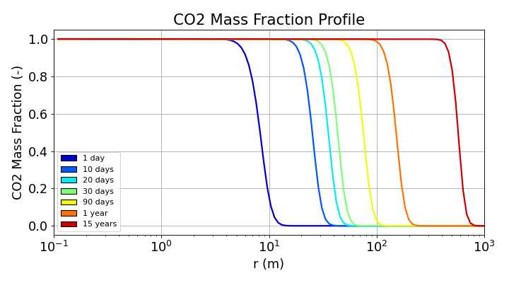
../../../../../../_images/plot_joule_thomson_profile_plot_co2_fraction.png — Fig. 16 Radial profiles of the CO2 mass fraction in the gas phase at the output times. The sharp front moves from about 9 m (1 day) to 550-600 m (15 years).

Pressure

The pressure build-up is largest at the injector and is concentrated in the first tens of meters at early times. At the first cell ( $r \approx 0.1$ m), the pressure is about 64 bar after 1 day, which is an increase of about 14 bar with respect to the initial pressure of 50 bar, and it rises slowly reaching 72 bar after 15 years (an increase of about 22 bar). In the region filled by CO2, the pressure decreases almost linearly with $\log r$ , with a drop of about 4-5 bar per decade of radius at 15 years.

The pressure perturbation travels much faster than the CO2 front, since it propagates by diffusion of the pressure (the compressibility of the gas is the only storage mechanism) while the front is transported with the fluid. After 1 day, the pressure is already perturbed up to about 30-50 m while the front is at 9 m, and after 1 year the whole domain is affected.

At the outer boundary, the pressure first decreases slightly below the initial value (about 49.7 bar after 1 year) because of the production, before the pressure wave of the injector arrives. It then increases to about 53 bar after 15 years: the system is closed and the injected mass (3 kg/s) is larger than the produced mass (0.56 kg/s), so that the average pressure of the reservoir increases. The pressure at the well is far below the 300 bar limit of the injector, which confirms that the injection stays at a constant rate.

(Source code)

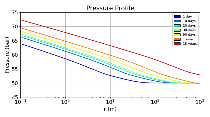
../../../../../../_images/plot_joule_thomson_profile_plot_pressure.png — Fig. 18 Radial profiles of the pressure at the output times. The pressure is highest at the injector (about 72 bar after 15 years) and tends to the initial value of 50 bar far from the well at early times.

Temperature and comparison with the paper

The temperature profiles show the three zones that are expected for this problem. Near the well ($r=0.1$ m), the injected gas has not yet expanded significantly, maintaining an elevated temperature of approximately 43 °C. Moving outward, JT expansion cools the gas and creates a temperature minimum. This minimum deepens and shifts farther from the well over time: after 1 day, the temperature drops to about 38.5 °C near 0.7 m. After 15 years, the minimum falls to roughly 31 °C at 30-40 m. Farther into the reservoir, the temperature recovers to the undisturbed baseline of 45 °C.

The cold region is much smaller than the region invaded by the CO2: after 15 years the temperature is back to about 45 °C beyond 100-150 m, while the CO2 front is at 550-600 m. The thermal front is retarded with respect to the gas front by the heat capacity of the rock and of the immobile water, which have to be cooled before the cooling can move forward. This is the transient effect mentioned above: the matrix attenuates the cooling, but the thermal front keeps propagating, and the minimum temperature keeps decreasing because the pressure drop that drives the JT cooling increases with time. The weak undershoot below 45 °C (a few tenths of a degree) at 15 years between the thermal front and the CO2 front is the cooling due to the small pressure drop in this region.

The magnitude of the minimum temperature is larger than a simple estimate based on the JT coefficient at the initial conditions. The pressure difference between the well and the location of the minimum at 15 years is about 10 bar (72 bar at the well, 61-62 bar at 30-40 m), so that a cooling of 14 °C requires an apparent JT coefficient of at least 1.4 K/bar, larger than the 0.9 K/bar of CO2 at 45 °C and 50 bar. This is consistent with the strong increase of $\mu_{JT}$ when CO2 approaches its critical point (31 °C and 73.8 bar), which is the case in the cold region, and it means that the cooling is sensitive to the thermodynamic model.

(Source code)

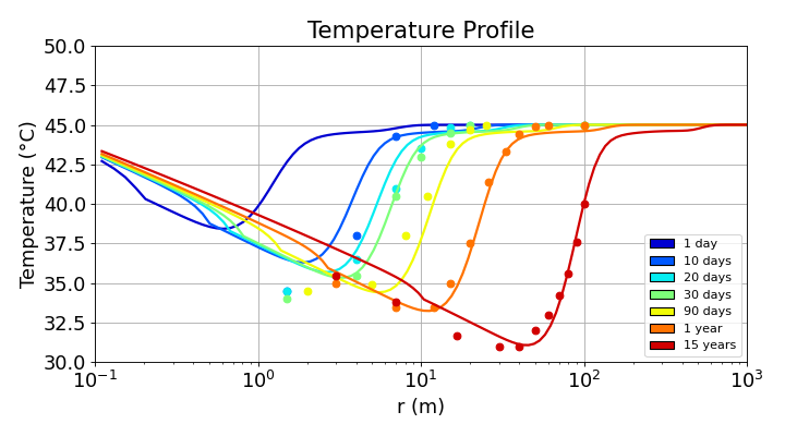
../../../../../../_images/plot_joule_thomson_profile_plot_temperature.png — Fig. 20 Radial profiles of the temperature at the output times (lines: *GEOS*; dots: results of Figure 7 of Oldenburg (2007), digitized). There is no reference curve for 1 day. The minimum temperature after 15 years (about 31 °C at 30-40 m) is reproduced, while *GEOS* is warmer than the paper close to the well (r < 10 m).

The comparison with the points taken from (Oldenburg, 2007) (dots) shows a good overall agreement, with some differences that are worth noting:

Good agreement on the cold front and on the minimum temperature. The position and the steepness of the thermal front are close to the digitized points at all times (for instance the rise from 35 to 45 °C between about 10 and 30 m after 1 year, and from 35 to 40 °C between about 60 and 100 m after 15 years), and the minimum temperature after 15 years, about 31 °C at 30-40 m, is the same as in the paper. This minimum is the quantity that matters for the risk of hydrate or ice formation, and it remains far above the temperature of hydrate stability. The thermal front and the CO2 front also have the same relative position as in the paper (the cooled zone stays inside the CO2-rich region).
Warmer temperatures in the near-well region. For $r$ smaller than about 10 m, the digitized points are lower than the GEOS curves. At early times (10 to 90 days), the paper gives 34-35 °C at 1.5-3 m, about 2 °C below the GEOS curves, and after 15 years the paper gives 35.5 °C at 3 m and 33.8 °C at 7 m, while GEOS is about 3-4 °C warmer. The paper also shows a minimum that is more flat and more extended (about 31-34 °C between 7 and 40 m at 15 years), whereas the GEOS profile decreases almost linearly with $\log r$ up to about 10 m and then drops more rapidly toward the minimum. GEOS therefore predicts a weaker cooling than the paper in the first meters around the injector.

Note

The cooling can be compared with the upper bound $\mu_{JT}\,\Delta P$ . The relevant pressure difference is the one between the well and the point of interest, and not the total pressure increase at the well, since the gas is injected at the reservoir temperature and cools as it expands toward lower pressures. As discussed above, the cooling observed in the simulation corresponds to an apparent JT coefficient larger than the one at the initial conditions, because of the proximity of the critical point, even though the heat released by the matrix, which is important in the first days and progressively exhausted, attenuates the cooling.

To go further

The other cases of the paper can be obtained from this input by changing a few parameters:

the permeability (rockPerm): $10^{-13}$ and $10^{-14}$ m² for Figures 5 and 6, and the summary of Figure 8; the injection rate is kept unchanged, so the pressure drop and the JT cooling vary with the permeability;
the porosity (rockPorosity), to study the compensation between the permeability and the heat supplied by the matrix (Figure 9);
the injection temperature and the initial reservoir temperature (injectionTemperature, initialTemperature) for the cases of Figures 10 and 11 (20 °C injection in a 75 °C reservoir). The initial compositions must then be computed again, as explained above.

Feedback on this example

For any feedback on this example, please submit a GitHub issue on the project’s GitHub page.

References

Oldenburg, C. M. 2007. Joule-Thomson cooling due to CO2 injection into natural gas reservoirs. Energy Conversion and Management, 48(6), 1808-1815. https://doi.org/10.1016/j.enconman.2007.01.010
Lemmon, E. W., McLinden, M. O., and Friend, D. G. 1998. Thermophysical Properties of Fluid Systems. In NIST Chemistry WebBook, NIST Standard Reference Database, eds. Linstrom, P. J. and Mallard, W. G., Vol. 69. Gaithersburg, Maryland, USA: National Institute of Standards and Technology. https://webbook.nist.gov/chemistry/fluid/